This is the follow up of the last post on Fraud Detection Overview. In this article, we will concentrate on the time series data and some methods to find outliers in time series data

Time series data

What is a time series data

Time series is defined as a collection of data points which is observed over a continuous time interval. Time series data is often used to find the changes of data over time. For example, we can measure how much calories we have burned every day to see if how fit we are; we could also calculate the money we have spent each day to find our spending behaviours; …

The above figure if an example of time series data (illustrated by the line chart on the right).We could also identify many other features in the graph. For example, looking at the graph, we could find that after 5 years, the value of Euro has been reduced ( from 30.000 VND to 25.000 VND). Moreover, there were some drastic changes at the end of 2014 (which corresponds to their crisis). Even the trend of data in last year could also be identified.

What is an outlier in time-series data

In the last post, we defined an outlier as “an observation point that is distant from other observations”.  As mentioned in the last section, using time series data we could detect the moving trend of data over time. Combine those two, an outlier in time series data is a data point which is distant from the overall trend of the whole dataset.

Using the above definition, we could create a general method to find outlier in time series data as follows:

• Collect time series data with noises and outliers. Normalize the value data
• Find the overall trend of data
• Identify the points which do not follow the overall trend ( points that are too distant to the estimated values according to the overall trend)

Detecting outlier in Time series data

There are many ways to calculate the moving trend of data. In this section, we will talk about two methods: moving average and regression.

To illustrate the algorithm, let’s define the input data. Assume that we are given:

• x[1], x[2], …, x[n] : the timestamp data (this could be a vector too)
• y[1], y[2], …, y[n] : the observed values (scalar)
• {x[i], y[i]} is a data point pair in which y[i] is observed at timestamp x[i]
• Y = {y[1], y[2], …, y[n]}^T : is the output vector
• X = {x[1], x[2], …, x[n]}^T : is the input vector

Moving average

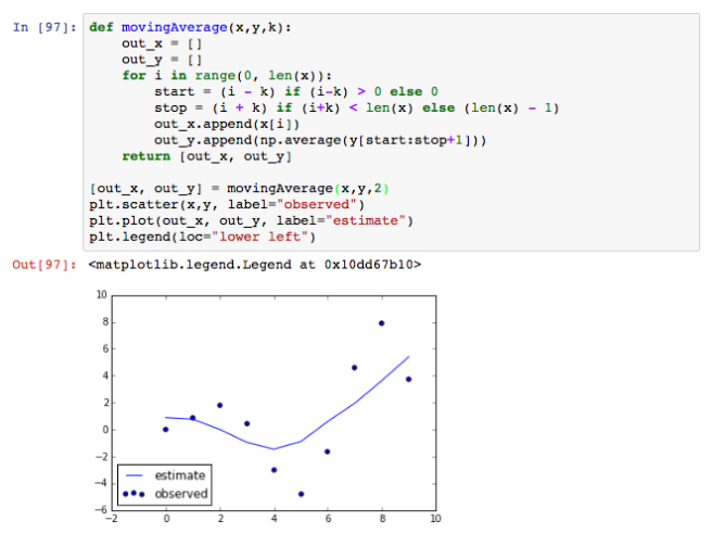
Moving average is one of the simplest methods to calculate and visualize the trend of time series data. Its idea is simple, the corresponded value of a timestamp is calculated as the average value of the surrounding points.

For instance, let 2k be the windows of the moving average. at timestamp x[i] we can calculate y[i] as:

Apply this equation to all the given points {x[i],y[i]} we achieve the estimated values of every timestamp.

Finding outlier in the given data now is quite simple. Just predefine a threshold and then identify all the data point j that have:

Note:

• Using surrounding points is not a must. We could also use k points that is observed before (or after) the selected point.
• There are several improvements for moving average algorithm. You can find them here

Median filter

Moving average offers an easy way to estimate and visualise the trend of time-series data. However, it has a big drawback which is: outlier often introduces a drastic change into the average value. Because of that, you may end up detecting some data points that are should not be filtered. Luckily, Median filter could solve this problem by estimating the observed values as the median of the surrounding values.

In other words, we have:

Similar to moving average, we now have to define a threshold and then find the outlier according to the threshold.

Both moving average and median filter have to face the same problem: they cannot provide an effective way to predict the value in the future because we do not have data in the future. For instance, The value of Euro compared to VND is rising according to the graph in the last section. Applying the moving average or median filter algorithms for the next step will result it a predicted value that is lower than the last measured time. Hence, the predicted value will not follow the overall trend of the data. To solve this problem, we can use the regression method.

Regression

Unlike moving average and median filter, regression calculates the relationship between every pair of observed data in the dataset.

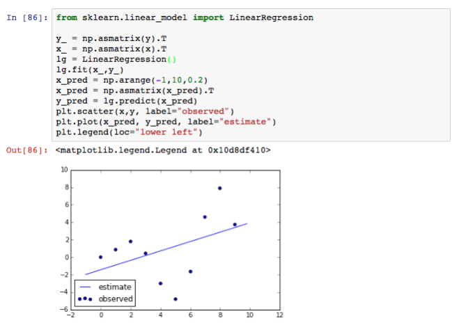
Among regression methods, linear regression is considered as the easiest method. It simply estimates a straight line that can be considered as the moving trend of data. In other words, we try to estimate a line which is:

Given the data, we can calculate the error rate:

and the total error is:

Minimising the total error yields

Outlier detection with Gaussian Process

Linear regression provides a method to find the moving trend of data. However, it is only a straight line. In real world data, we have seen many data that should not be estimated as a straight line. The currency graph above is an example. Therefore, we need a better regression method that not only capture the nature of the given dataset, but also robust to the noise (or outlier)

Gaussian Process is a nonparametric method to discover the trend of data. It also offer a good probabilistic model that is robust to the input noise (which can be considered as outlier).

Let’s move the the algorithm of Gaussian Process itself. In gaussian process we assume that“data points are a collection of random variables, any finite number of which have a joint Gaussian distribution”  – Rasmussen.

Similar to Gaussian Distribution, Gaussian Process is defined by its mean function and covariance function. They can be calculated as:

At this moment, a gaussian process is controlled by the covariance function. Let’s consider the most common covariance function: RBF function (or Gaussian function). In RBF function, k(x[i], x[j]) is calculated by the following equation:

In which

Assume that we want to predict the value y[m] at x[m]. We need to prepare

Then, we can calculate the predicted y[m] by:

with variance:

Note that: all the parameters of the gaussian process can be learned from the given data using marginal gradient ascent method.

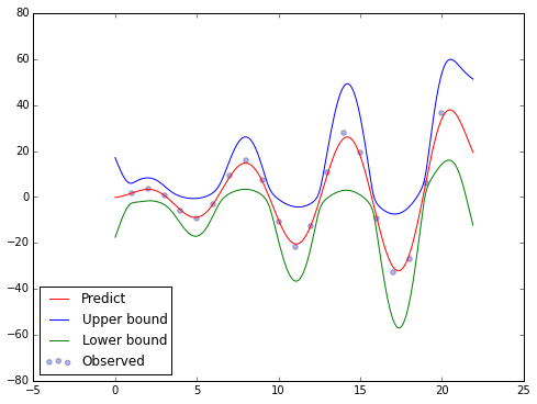
In statistic, we have the 67-95-99.7 rule. Applying this rule into our problem we will have the predictive confidence of y[m]. This also helps us to identify the outlier in the data (the observed data does not stay inside the selected confidence interval of the predicted da

Example

Input data

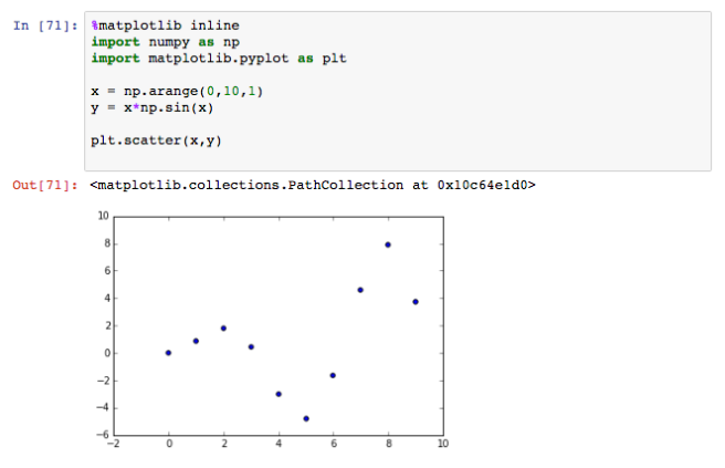
Let’s create an input using python

Moving average

Median filter

Linear regression

Gaussian process